![[Rod Stephens Books]](banner_300x110.png)
|
|
|
![[Build Your Own Python Action Arcade!]](book_action_arcade_80x100.jpg)
![[Build Your Own Ray Tracer With Python]](book_python_ray_tracer_81x100.png)
![[Beginning Database Design Solutions, Second Edition]](book_db2_79x100.png)
![[Beginning Software Engineering, Second Edition]](book_sw_eng2_79x100.png)
![[Essential Algorithms, Second Edition]](book_algs2e_79x100.png)
![[The Modern C# Challenge]](book_csharp_challenge_80x100.png)
![[WPF 3d, Three-Dimensional Graphics with WPF and C#]](book_wpf3d_80x100.png)
![[The C# Helper Top 100]](book_top100_80x100.png)
![[Interview Puzzles Dissected]](book_interview_puzzles_80x100.png)

Title: Draw a Hilbert curve fractal with Python and tkinter
When you click the program's Draw button, the following code executes. def draw(self): # Delete any previous drawing objects. self.canvas.delete(tk.ALL) # Get the desired depth. try: depth = int(self.depth_var.get()) except: messagebox.showinfo('Depth Error', 'Depth must be an integer between 1 and 10.') return if depth < 1 or depth > 10: messagebox.showinfo('Depth Error', 'Depth must be an integer between 1 and 10.') return # See how big we can make the curve. wid = self.canvas.winfo_width() hgt = self.canvas.winfo_height() total_length = min(wid, hgt) - 20 start_x = (wid - total_length) / 2 start_y = (hgt - total_length) / 2 # Compute the side length for this level. dx = total_length / (2 ** depth - 1) dy = 0 # Create the points list. points = [(start_x, start_y)] hilbert(points, depth, dx, dy) # Draw the polygon. self.canvas.create_line(points, width=1, fill='black') This code first gets the desired depth of recursion and makes sure it's a reasonable value. It then gets the canvas's dimensions and calculates the length of the segments that will make up the curve. If you experiment with the program for a while, you can see that a curve of depth D is 2D - 1 segments wide and tall, so the program calculates the segment length by dividing the available space by 2D - 1. (You can also prove this fairly easily by induction. Perhaps I'll make that another post.)The code then sets dx and dy so they draw the first segment to the right. It creates a points list and then calls the hilbert method shown shortly to do all of the really interesting work. After the hilbert method has added all of the points to the points list, the program adds a Line shape to its Canvas widget to display the curve as a single long multi-line.
The following code shows the hilbert method. def hilbert(points, depth, dx, dy): '''Add points to draw a hilbert curve.''' if depth > 1: hilbert(points, depth - 1, dy, dx) draw_relative(points, dx, dy) if depth > 1: hilbert(points, depth - 1, dx, dy) draw_relative(points, dy, dx) if depth > 1: hilbert(points, depth - 1, dx, dy) draw_relative(points, -dx, -dy) if depth > 1: hilbert(points, depth - 1, -dy, -dx) This amazingly short piece of code draws the curve. First, if the current depth of recursion is greater than 1, the code calls itself recursively to draw a depth - 1 level curve. It then uses the draw_relative method described shortly to draw a segment (which is red in the picture) connecting that smaller curve to the next one. The code repeats those steps to draw three more depth - 1 level curves, connecting them to the previous ones.Notice how the recursive calls change the dx and dy parameters to create the sub-curves with the proper orientations. The following code shows the draw_relative method. def draw_relative(points, dx, dy): '''Add (dx, dy) to the last point in the points list.''' points.append( (points[-1][0] + dx, points[-1][1] + dy)) This method adds a new point to the point's list. Each point is a two-item list holding a point's X and Y coordinates.Each point is relatively to the previous one, so it is offset (dx, dy) from the position of the last point currently in the list. To place the new point, the code uses the list slices [-1][0] and [-1][1] to get the X and Y coordinates of the last point in the list. It adds the dx and dy values, and adds the result to the points list. Download the example to experiment with the program and to see all of the details. |
![[This program draws a Hilbert curve fractal with Python and tkinter]](hilbert_curve.png)
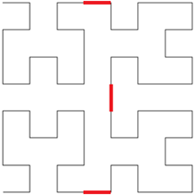 The key to drawing the Hilbert curve is to use smaller curves that are rotated and positioned appropriately to make up larger curves. The picture on the right shows a depth 3 curve made up of smaller depth 2 curves. The depth 2 curves are drawn with thin black lines and they are connected with thick red lines.