My book Build Your Own Ray Tracer With Python explains how to draw amazing ray traced images with Python including one of those shown here. It's very cool, although much slower than using MatPlotLib and Numpy.

Title: Plot a three-dimensional surface with Python, Matplotlib, and NumPy

[This program plot a three-dimensional surface with Python, Matplotlib, and NumPy]

I love programming, particularly graphics programming such as drawing fractals and three-dimensional shapes. I find it immensely satisfying to dump a bunch of numbers into a program and have a beautiful image pop out. Often when I need a pick-me-up, I turn crank out a new fractal or 3-D program, and that's what I did here.

This program plots the following weird three-dimensional surface. (It's one of my favorite three-dimensional equations because it's so strange.)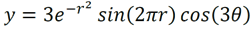

There are many ways that you can plot three-dimensional surfaces. For example, you can write your own three-dimensional graphics program or a ray tracer. The green picture on the right shows the result of one of the programs in my book Build Your Own Ray Tracer With Python.

Unfortunately, ray tracing is notoriously slow. Really slow! I don't remember exactly how long my ray tracer took to generate that picture, but it was probably a few hours.

Ray tracers can produce all sorts of cool effects like shadows (which you can see in the picture), reflections, textures, translucency, depth of field, ambient occlusion, and more. If you don't need those fancier features, there's a much faster way to draw this kind of three-dimensional surface: Matplotlib.

This program's code is fairly short, but it is confusing because it assumes you know a fair bit about Matplotlib functions. Don't worry, after you look at the code, I'll walk you through it. (If you're comfortable with Matplotlib and the code is obvious to you, just skip to the end.)

import math import matplotlib.pyplot as plt import numpy as np # Create a figure and a 3D axes object fig = plt.figure(figsize=(10, 10)) # Size the figure (inches) ax = plt.axes(projection='3d') # Generate some data for the graph num_divisions = 1000 x = np.linspace(-2, 2, num_divisions) y = np.linspace(-2, 2, num_divisions) X, Y = np.meshgrid(x, y) approach = 1 if approach == 1: Z = 3 * np.exp(-(X * X + Y * Y)) * \ np.sin(2 * np.pi * np.sqrt(X * X + Y * Y)) * \ np.cos(3 * np.arctan2(Y, X)) elif approach == 2: function = lambda x, y: \ 3 * math.exp(-(x * x + y * y)) * \ math.sin(2 * math.pi * math.sqrt(x * x + y * y)) * \ math.cos(3 * math.atan2(y, x)) z = [[function(x_value, y_value) for x_value in x] for y_value in y] Z = np.array(z) # Plot the surface # For info on color maps, see https://matplotlib.org/stable/users/explain/colors/colormaps.html # Add _r at the end of a color map name to reverse its colors. # Note that color map names are case-sensitive (for some reason). surf = ax.plot_surface(X, Y, Z, cmap='viridis') # Add a colorbar to the plot fig.colorbar(surf, shrink=0.5, aspect=5) # Set labels for the axes ax.set_xlabel('X') ax.set_ylabel('Y') ax.set_zlabel('Z') ax.view_init(elev=15, azim=20) # Set elevation and azimuth (degrees) # Show the plot plt.show()

The code begins with some imports. Matplotlib will do the actual drawing but it uses NumPy to represent arrays and to perform some calculations.
After importing libraries, the code calls Matplotlib's figure function to create a new figure. The code sets the figure's size to 10" × 10" so it's not too small. For more information about the figure function including about 160 example programs, see the matplotlib.pyplot.figure documentation.
Next, the code uses axes to get an axis for the figure. An axis represents a sub-plot, in this case the sub-plot that will hold the actual surface. The projection='3d' part indicates that we will be making a three-dimensional plot.
Now the code sets num_divisions to 1000. That will be the number of divisions the surface uses in the X and Y directions, so the final plot will use a total of 1000 × 1000 = 1 million data points.
The code then sets x = np.linspace(-2, 2, num_divisions). This tells NumPy to make a linear (one-dimensional) array holding num_divisions values ranging from -2 to 2. The code repeats that step to make a similar array so x and y now hold coordinates for the points that we will plot.
Next, the program calls NumPy's meshgrid function to expand the two one-dimensional x and y arrays. It does that by making two new two-dimensional arrays containing the values in x repeated len(y) times and the values in y repeated len(x) times. Yes, this is pretty confusing.
Imagine that you want to make a grid with X values [1, 2, 3] and Y values [a, b] sort of like this:
1 2 3 a . . . b . . .
The meshgrid function fills in values so the program can later look up X and Y values for every point in the grid. To do that, it creates arrays holding the X and Y coordinates for every point in the grid. Here's a small program (plus its output) that shows how this works for this mini-example.
x = [1, 2, 3] y = ['a', 'b'] X, Y = np.meshgrid(x, y) print(X) print(Y) [[1 2 3] [1 2 3]] [['a' 'a' 'a'] ['b' 'b' 'b']]
Now to find the X and Y values at position (i, j), you can look at X[i][j] and Y[i][j].
Now back to the program's code. Having expanded the x and y values into X and Y, the code takes one of two approaches to generate the Z values that go with the X and Y values.
Approach 1
The first approach uses NumPy to evaluate the weird function. It's faster than the second approach and therefore probably better, although you may find the second approach slightly more intuitive (at least if you're comfortable with list comprehensions).
Here's the code used by Approach 1 to initialize the Z array.
Z = 3 * np.exp(-(X * X + Y * Y)) * \ np.sin(2 * np.pi * np.sqrt(X * X + Y * Y)) * \ np.cos(3 * np.arctan2(Y, X))
This code evaluates the weird equation shown earlier. There are two strange things here. First, the code use X and Y, which are arrays, not simple numeric values. NumPy arrays are smart enough to evaluate operations like + and * component-wise so it uses the corresponding values in X and Y to produce a resulting matrix Z.
Unfortunately, the math library doesn't know how to do that so you can't use methods like math.sqrt in this sort of equation. Instead you need to replace any math calls to the corresponding NumPy calls. That's the second strange thing about this equation.
The result is a Z array that holds the values of the function for each of the X and Y values.
Approach 2
Here's the code the second approach uses to build the Z array.
function = lambda x, y: \ 3 * math.exp(-(x * x + y * y)) * \ math.sin(2 * math.pi * math.sqrt(x * x + y * y)) * \ math.cos(3 * math.atan2(y, x)) z = [[function(x_value, y_value) for x_value in x] for y_value in y] Z = np.array(z)
The code first creates a lambda function that evaluates the weird equation. This function uses normal math library functions instead of the NumPy versions.
The program then uses a list comprehension to loop over the values in the x and y lists, evaluates the function for those values, and stores the result in the new z list. For example, if i and j are values in the x and y lists, then the result holds the value function(i, j).
The result is a list of lists holding the Z values in the area of interest. Matplotlib uses work NumPy arrays not lists of lists, so the code calls NumPy's array function to convert the list of lists into a two-dimensional array.
Finishing the Plot
Having built the X, Y, and Z arrays, the program passes those arrays into the axis object's plot_surface method to generate the plot. The code tells that method to color the surface with the veridis color map. For a nice page that shows color examples of other color maps, see the Matplotlib page Choosing Colormaps in Matplotlib. As the comment in the code notes, the color map names are case-sensitive.
Next, the program adds a color bar to the figure. Comment out that statement if you don't want it. It also labels the figure's X, Y, and Z axes. Again, comment out those lines if you don't want the labels.
The code then calls ax.view_init to set the plot's viewing position. You can omit that statement if you want to accept the default viewing position.
The picture on the right shows the program with no color bar or axis labels shown from the default viewing position.
Finally, the program calls plt.show() to make the result actually appear.
Summary
As I said, this example's code isn't too long but it's a bit confusing if you're not familiar with Matplotlib. Hopefully you now know how to plot a three-dimensional surface and you understand a bit more about Matplotlib, NumPy arrays, and NumPy functions when applied to matrices.
Search online for more general information about Matplotlib and NumPy. See my book Build Your Own Ray Tracer With Python for information about ray tracing in Python.
And as always, download the example to see all of the details.