![[Rod Stephens Books]](banner_300x110.png)
|
|
|
![[Build Your Own Python Action Arcade!]](book_action_arcade_80x100.jpg)
![[Build Your Own Ray Tracer With Python]](book_python_ray_tracer_81x100.png)
![[Beginning Database Design Solutions, Second Edition]](book_db2_79x100.png)
![[Beginning Software Engineering, Second Edition]](book_sw_eng2_79x100.png)
![[Essential Algorithms, Second Edition]](book_algs2e_79x100.png)
![[The Modern C# Challenge]](book_csharp_challenge_80x100.png)
![[WPF 3d, Three-Dimensional Graphics with WPF and C#]](book_wpf3d_80x100.png)
![[The C# Helper Top 100]](book_top100_80x100.png)
![[Interview Puzzles Dissected]](book_interview_puzzles_80x100.png)

Title: Draw a Sierpinski curve fractal with Python and tkinter
This example shows how to build a Sierpinski curve fractal, a space-filling curve that is in some ways similar to the Hilbert curve fractal. Enter the desired maximum depth of recursion and click Draw to draw the curve. The curve is drawn by four methods named sierp_a, sierp_b, sierp_c, and sierp_d that draw curves across the top, right, bottom, and left sides of the area being drawn. The following code shows the sierp_a method. def sierp_a(points, depth, dx, dy): '''Draw right across the top.''' if depth > 0: depth -= 1 sierp_a(points, depth, dx, dy) draw_relative(points, dx, dy) sierp_b(points, depth, dx, dy) draw_relative(points, 2 * dx, 0) sierp_d(points, depth, dx, dy) draw_relative(points, dx, -dy) sierp_a(points, depth, dx, dy) 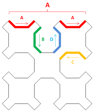 Each of the methods calls other methods to draw pieces of the curve (so these are multiply recursive methods). For example, sierp_a calls itself to draw a horizontal section, draws a line down and to the right, calls sierp_b to draw down, draws a horizontal segment, calls sierp_d, draws another segment, and finishes by calling sierp_a again. See the picture on the right.
Study the picture to figure out how the program draws the curve's other sides. For example, B = B + C + A + B. The following sierpinski method calls the four recursive methods to draw the finished curve. def sierpinski(points, depth, dx, dy): '''Draw a Sierpinski curve.''' x = 2 * dx y = dy sierp_a(points, depth, dx, dy) draw_relative(points, dx, dy) sierp_b(points, depth, dx, dy) draw_relative(points, -dx, dy) sierp_c(points, depth, dx, dy) draw_relative(points, -dx, -dy) sierp_d(points, depth, dx, dy) draw_relative(points, dx, -dy) The points parameter is the list that will hold the curve's points. Initially it contains the curve's starting point.The sierpinski method calls the four recursive methods, using the following draw_relative method to add the connecting segments between them. def draw_relative(points, dx, dy): '''Add (dx, dy) to the last point in the points list.''' points.append( (points[-1][0] + dx, points[-1][1] + dy)) This method simply adds dx and dy to the last point in the points list and appends the result to the list.The main program uses the following code to get the process started. # See how big we can make the curve. wid = self.canvas.winfo_width() hgt = self.canvas.winfo_height() # Compute dx and dy. margin = 10 curve_width = min(wid, hgt) - 2 * margin num_divisions = (2 ** (depth + 2)) - 2 dx = curve_width / num_divisions dy = dx start_x = (wid - curve_width) / 2 + dx start_y = (hgt - curve_width) / 2 # Create the points list. points = [(start_x, start_y)] sierpinski(points, depth, dx, dy) # Draw the polygon. self.canvas.create_line(points, width=1, fill='black') print(f'# points: {len(points)}') This code first gets the dimensions of the program's canvas. To determine how large to make the curve, it takes the minimum of the canvas's width and height and then subtracts twice the desired margin.
More generally, if the curve has depth D, then it has 2D + 2 - 2 divisions. The code divides the curve's width by the number of divisions to calculate the length and width dx of the divisions. Next, the program calculates where it should start the curve to center it on the canvas. It creates the points list, adding the starting point to it, and then calls the sierpinski method to build the curve's other points. Finally the code creates a line that connects the points to draw the curve. Download the example to see all of the details. |
![[A Sierpinski curve fractal]](sierpinski_curve.png)
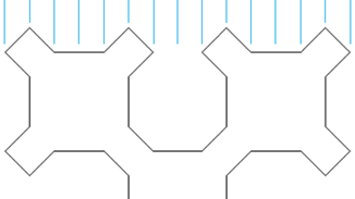 Next the program calculates the number of divisions the curve will have vertically and horizontally. The picture on the right shows the top of a depth 2 curve with the divisions marked. You can see that the depth 3 curve has 14 divisions. A depth 1 curve consists of only the left half of that picture and has 6 divisions.